ANN architectures: From Perceptron to Transformers
Collection of personal notes, sources and explanations.
Perceptron
Code examples:
FFNN
Sources:
Code examples:
RNN
Sources:
- The Unreasonable effectiveness of RNN: http://karpathy.github.io/2015/05/21/rnn-effectiveness/
Code examples:
- Minimal char-rnn in Numpy by Karpathy
- Minimal char-rnn in Keras
- Minimal char-rnn in Keras by me with more comments :)
Cell agnostic RNN variants
Dilated RNN
- https://arxiv.org/abs/1710.02224
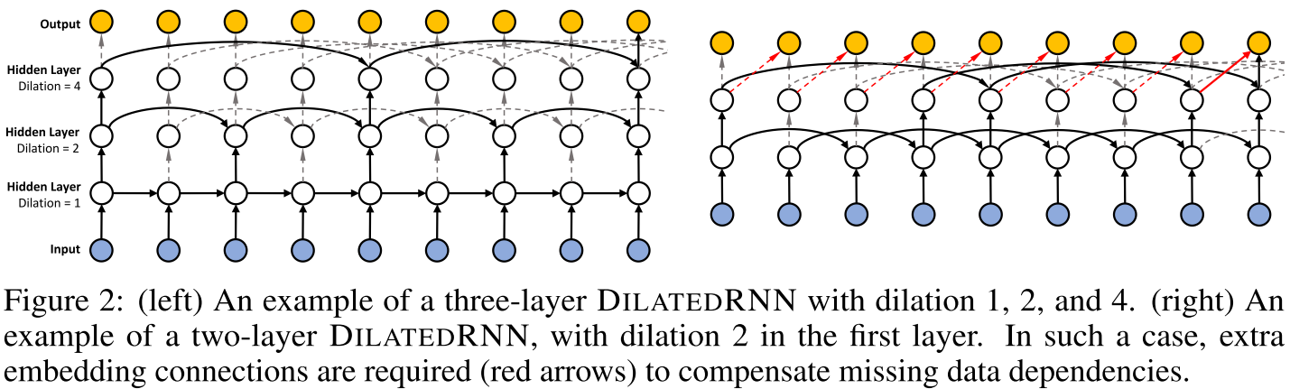
- difference to regular skip connection:
- skip connection layer =
f(x_t, c_{t-1}, c_{t-d})- the previous output is combined with the skip connection - dilated layer =
f(x_t, c_{t-d})- the previous output is not inputted
- skip connection layer =
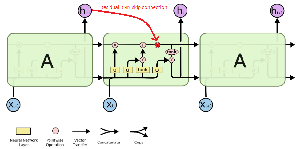
Residual RNN
- https://arxiv.org/abs/1701.03360
- use highway skip connection on hidden state
- or use skip connection on cell state
- or residual RNN:
- skip connection of h_{t-1} to cell state before hidden output
LSTM
Sources:
- Great blog by Distill founder: https://colah.github.io/posts/2015-08-Understanding-LSTMs/ = source of the diagrams!
- LSTM variants, hyperparam tuning etc.: LSTM: A Search Space Odyssey
Explanation:
- 1 LSTM layer = 1 LSTM cell = 1 box on the diagram
- 1 LSTM cell processes a sequences of vectors x_t and returns a sequence of vectors h_t
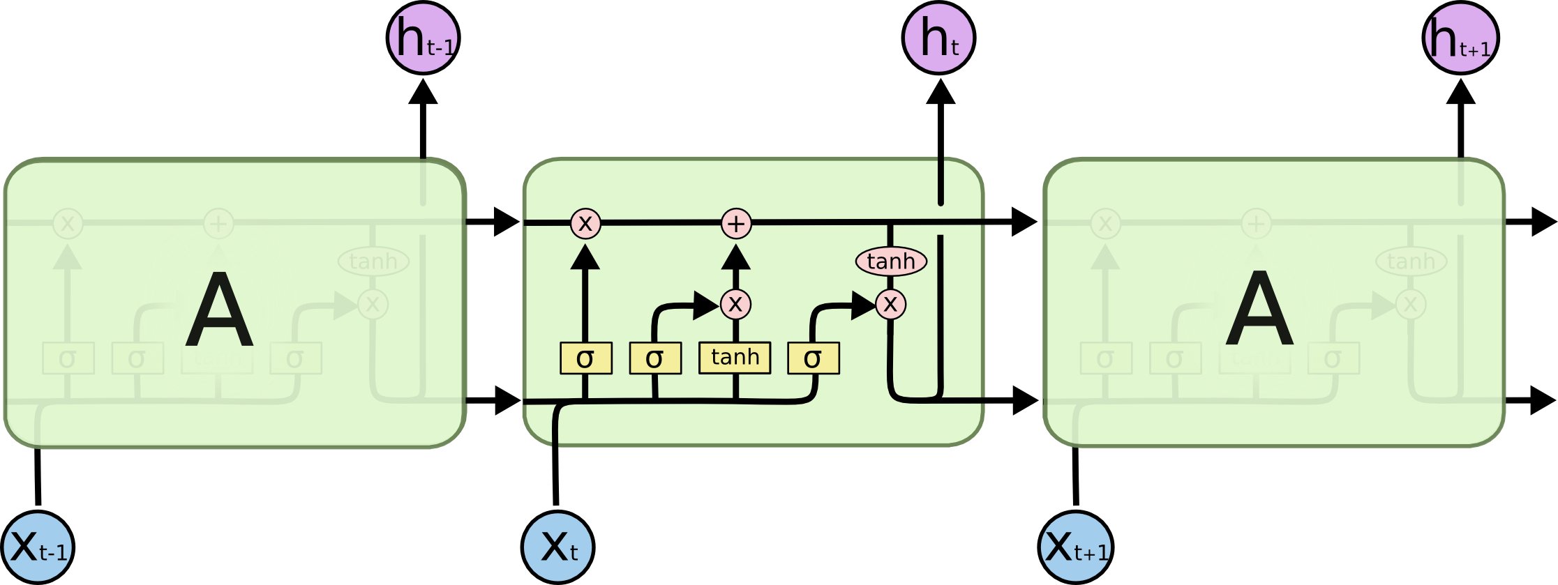
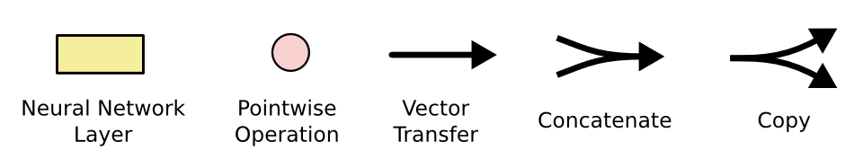
- Sigmoid/Tanh Neural Network Layer = densely connected feed-forward layer with Sigmoid/Tanh activation
- Sigmoid returns [0,1]
- Tanh returns [-1, 1] - used as normalization + has better gradients than Sigmoid
Stacked LSTM
model = Sequential()
model.add(LSTM(layer_size, return_sequences=True, input_shape=(3,1)))
model.add(LSTM(layer_size, return_sequences=True))
model.add(LSTM(layer_size, return_sequences=True))
model.compile(optimizer='adam', loss='mse')
- The first LSTM layer LSTM_0 gets input sequence X and return a sequence S_1
- The second LSTM layer LSTM_1 gets input S_1 and outputs a sequence S_2 etc.
- It can be imagined as the LSTM cell unrolled in time with another one on top of it with x_t replaced by h_t of the first LSTM layer:
- x_0 -> LSTM_0 -> h_0_0 -> LSTM_1 -> h_0_1 -> … -> first element of output sequence
- x_1 -> LSTM_0 -> h_1_0 -> LSTM_1 -> h_1_1 -> … -> second element of output sequence
Sequence-to-Sequence architectures: (mainly from machine translation POV)
Sources:
Attention seq2seq models from translation:
seq2seq learning:
- Sequence to Sequence Learning with Neural Networks
- Learning Phrase Representations using RNN Encoder-Decoder for Statistical Machine Translation
- TensorFlow Neural Machine Translation (seq2seq) Tutorial
- Blogpost - source for seq2seq image
Sequence Modeling:
- = predict after each time step: x_t -> y_t
- predictions based only on the previous elements in the sequence
- Dilated Convolutions (TCN = Temporal Convolutional Nets) VS RNN:
- Paper: https://arxiv.org/abs/1803.01271
- Code by authors: https://github.com/locuslab/TCN
- My talk + handout: https://github.com/BartyzalRadek/lets-talk-ml/blob/master/talks/CNN_vs_RNN
Sequence-to-Sequence:
- process whole input sequence and then generate the new sequence
- e.g. machine translation
Encoder-Decoder architecture
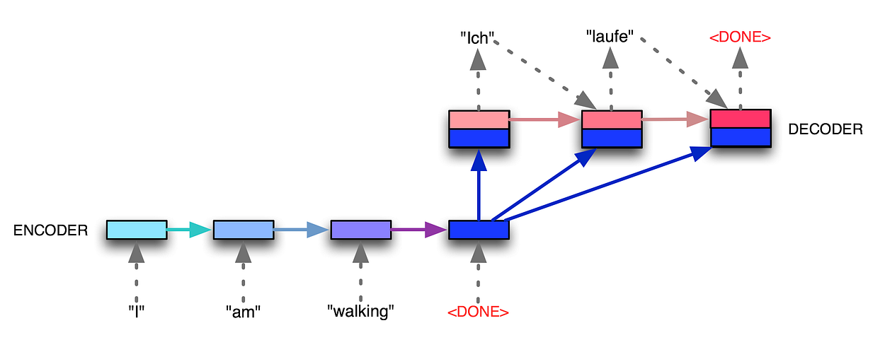
Encoder-Decoder with fixed-size context vector (source)
- Encoder = RNN: processes whole input sequence and outputs a single fixed-size context vector C representing it
- Decoder = RNN: at each time step t:
- input: C and h_{t-1}
- output: h_t = hidden representation at time t that is then passed through a FFNN to get distribution over classes (characters, words, etc..)
- Encoder and Decoder can but usually don’t share their weights
- input does not have to be a sequence: generate text descriptions for images:
- Encoder = CNN outputting context vector
- Decoder = RNN generating text from the.md
- Show and Tell: A Neural Image Caption Generator
Encoder-Decoder with Attention
- containing all information about a long input sequence in one fixed-size vector is hard => attention
- save all the hidden states of the encoder not just the last one (previously called C)
- context is now a list of hidden states (or RNN outputs) with same length as the input sequence = input_seq_len * RNN_output_dim matrix
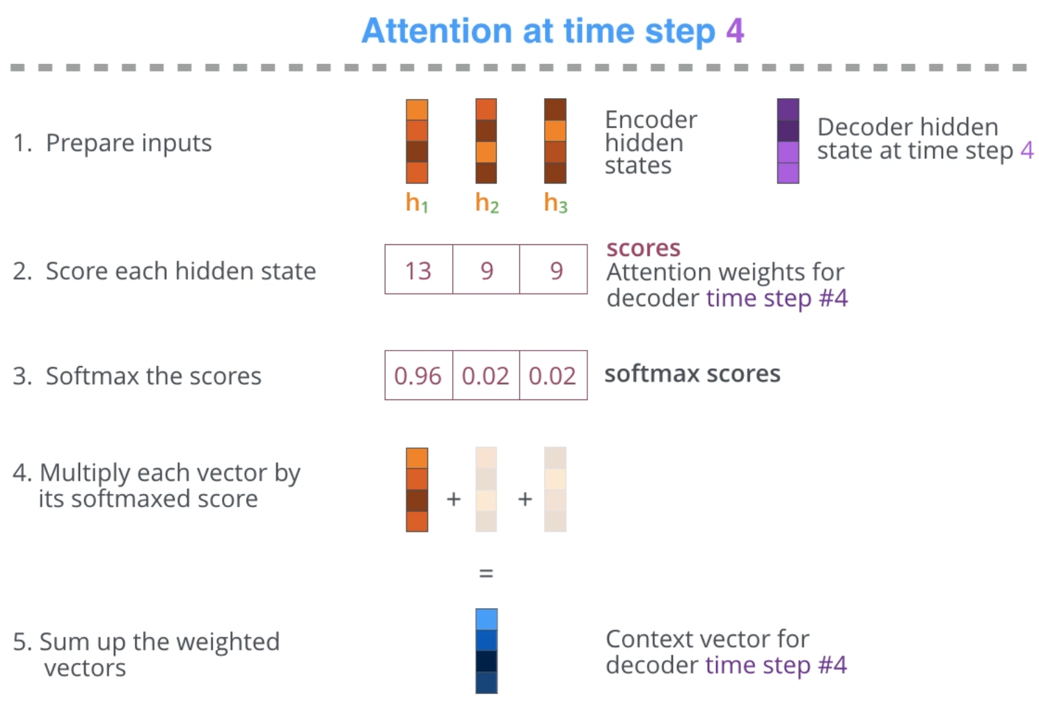
- Decoder = RNN: at each time step t:
- process the context list into a single fixed-size vector by attention
- = weighted sum over the hidden states - the weights are generated at each step = focus on different parts of the input
- input:
- processed context = single RNN_output_dim sized vector
- h_{t-1}
- output: h_t = hidden representation at time t that is then passed through a FFNN to get distribution over classes (characters, words, etc..)
- Attention calculation at time step = 4 = input sequence has length 3 = we have 3 hidden states from encoder and now we are decoding:
Transformer
- Orig paper: Attention Is All You Need
- pytorch impl. with a blogpost
- tensor2tensor library with official implementation of Transformer in TF
- Illustrated Transformer = source for used imgs
- Transformer talk by author - source for motivation
- Motivation:
- RNNs:
- not parallelizable
- number of time steps = input sequence length
- possibly a lot of words between words relevant to each other
- O(n * d^2) - n = input seq length, d = hidden representation dimension
- Dilated Convolutions CNNs:
- parallelizable
- log(n) number of time steps with input sequence length n
- still too focused at the position of the words
- O(n * d^2) - n = input seq length, d = hidden representation dimension
- Transformer:
- Encoder calculates word embeddings in constant number of time steps
- Decoder can generate whole sequence in constant number of steps during training
- Decoder outputs one element of output sequence at a time during inference = its sequential
- O(n^2 * d) - worse in theory but in machine translation: d =~1000, n=~100 => 10x faster than RNN
- RNNs:
- Whole architecture:
- Feed Forward layers at the same level share weights = it just one layer depicted as 2 to show that the comp. can be parallelized there
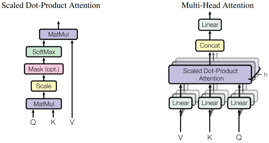
- FF layer = two linear transformations with ReLU in between =
ReLU(W_1*x + b_1) * W_2*x + b_2- dim(W_1) = 2048, dim(W_2) = 512 = token dim
- Add + Normalize = LayerNorm(layer_output + residual_connection)
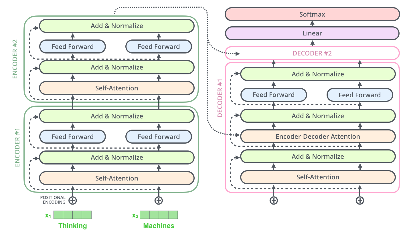
- Encoder:
- Self attention:
- Q, K, V = input embeddings * W_Q, W_K, W_V = Linear layer
- Q, K, V can all be identical!
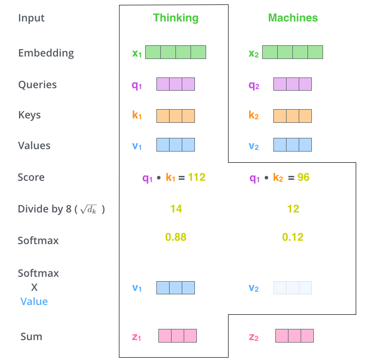
- In matrix form:
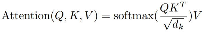
- Multi-head attention = multiply Q, K, V by Linear layer to make them smaller -> do the self attention 8 times -> concat outputs -> multiply by W_O to get output of correct shape = Linear layer:
- Decoder:
- First input is
starttoken - Rest of inputs is the translated sentence = labels shifted to the right =
teacher forcing - To prevent model from looking at the labels = Masked Self-Attention = words can look only at previous words during self-attention
- Inference = generate a new sentence:
- Insert
starttoken or embedding based on Encoder output - Outputs a prob. distrib. over words
- get most likely word:
- greedy inference = select the one with highest prob
- beam search = get N words with highest prob and input them to see which ones generate smaller error
- Append generated word to input sequence and generate a new word
- Insert
- First input is
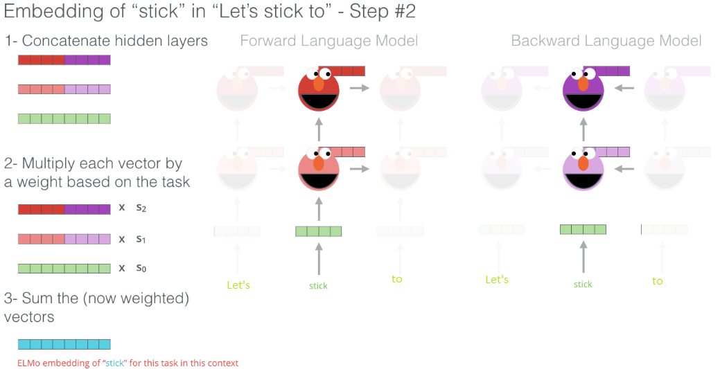
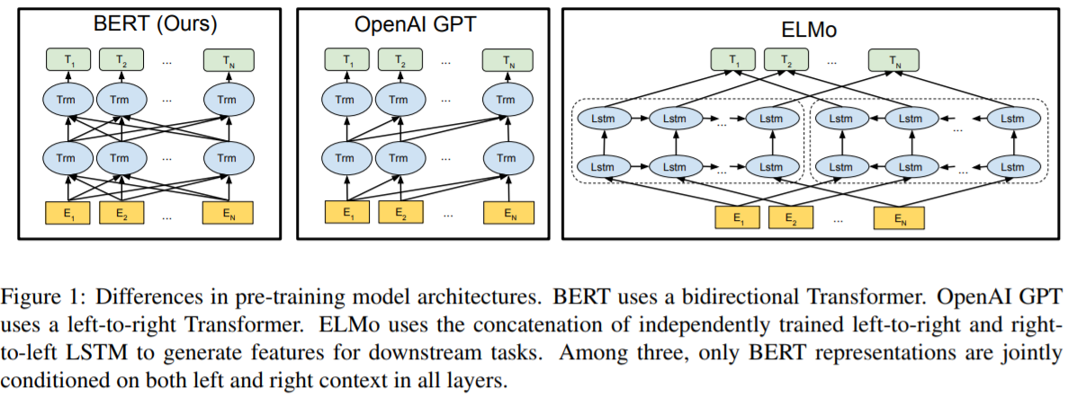
ELMo = Embeddings from Language Models
- Deep contextualized word representations
- https://jalammar.github.io/illustrated-bert/
- uses bi-directional LSTM - concats their hidden repr.
- pretrained on large unsupervised text corpora - predict the next word = dense + softmax layer on top of last LSTM layer output
- outputs contextual word embeddings - these can be used in further tasks
- no finetuning necessary just append task specific architecture on top of pretrained ELMo and train only the added part
OpenAI GPT = Generative Pre-trained Transformer
- https://openai.com/blog/language-unsupervised/
- GPT2 - https://openai.com/blog/better-language-models/
- just Transformer decoder
- unsupervisely trained on predicting next word of sequence
- decoder already masks the next words = can’t look at them during attention
- left-to-right language model = looks only at past words
- all words are predicted = gradient flows through all “vertical paths” = token embeddings
BERT = Bidirectional Encoder Representations from Transformers
- different BERT versions simply explained as git diffs: https://amitness.com/2020/05/git-log-of-bert/
- Pre-trained models + src = https://github.com/google-research/bert
- BERT: Pre-training of Deep Bidirectional Transformers for Language Understanding
- transformer encoder = they call it bi-directional, it’s all-directional = attention
- jointly conditioning on both left and right context in all layers = normal transformer encoder:
- not just concat like ELMo
- not left-to-right like Open AI GPT = Transformer decoder trained to predict next word in sequence
- pre-trained on:
- predicting masked words = 15% of input sequence = not just the next word like ELMo/GPT
- only 15% of words have error = gradient, unlike GPT where all words have error
- slower training but the benefit of looking at whole input sequence = overcomes GPT in couple epochs
- predict whether 2 sentences follow each other
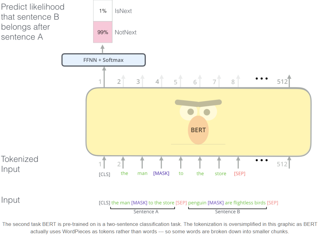
- input:
- input token = token + segment embedding + positional embedding
- use WordPiece embeddings
- learned positional embeddings with supported sequence lengths up to 512 tokens
- first token is always [CLS] = output of encoder on this token is input sequence embedding inputted to classification layers
CNN
Sources:
Notes:
-
For example, suppose that the input volume has size [32x32x3], (e.g. an RGB CIFAR-10 image). If the receptive field (or the filter size) is 5x5, then each neuron in the Conv Layer will have weights to a [5x5x3] region in the input volume, for a total of 5x5x3 = 75 weights (and +1 bias parameter). Notice that the extent of the connectivity along the depth axis must be 3, since this is the depth of the input volume. = The connectivity is local in space (e.g. 5x5), but full along the input depth (3).
-
Parameter sharing: We are going to constrain the neurons in each depth slice to use the same weights and bias.
- WxHxD = size of input
- F = filter size
- K = number of filters
With parameter sharing, it introduces F⋅F⋅D weights per filter, for a total of (F⋅F⋅D)⋅K weights and K biases for the whole network.
-
1x1 convolution: If the input is [32x32x3] then doing 1x1 convolutions would effectively be doing 3-dimensional dot products (since the input depth is 3 channels).
-
Dilated convolutions: Dilation of 0:
w[0]*x[0] + w[1]*x[1] + w[2]*x[2]. For dilation 1 the filter would computew[0]*x[0] + w[1]*x[2] + w[2]*x[4]. If you stack two 3x3 CONV layers on top of each other then you can convince yourself that the neurons on the 2nd layer are a function of a 5x5 patch of the input (we would say that the effective receptive field of these neurons is 5x5). If we use dilated convolutions then this effective receptive field would grow much quicker.- My talk explaining dilated convs vs RNN: https://github.com/BartyzalRadek/lets-talk-ml/blob/master/talks/CNN_vs_RNN
-
Pooling: Pooling layer with filters of size 2x2 applied with a stride of 2 downsamples every depth slice in the input by 2 along both width and height, discarding 75% of the activations.
-
Getting rid of pooling: Discarding pooling layers has also been found to be important in training good generative models, such as variational autoencoders (VAEs) or generative adversarial networks (GANs).
-
Simple layer pattern:
INPUT -> [[CONV -> RELU]*N -> POOL?]*M -> [FC -> RELU]*K -> FC -
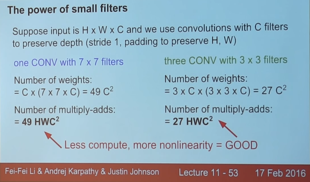
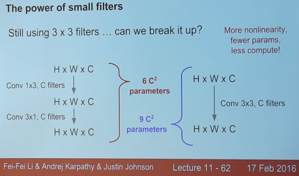
Prefer a stack of small filter CONV to one large receptive field CONV layer.
The neurons would be computing a linear function over the input, while the three stacks of CONV layers contain non-linearities that make their features more expressive.
Intuitively, stacking CONV layers with tiny filters as opposed to having one CONV layer with big filters allows us to express more powerful features of the input, and with fewer parameters. As a practical disadvantage, we might need more memory to hold all the intermediate CONV layer results if we plan to do backpropagation.
-
Why are smaller filters better than larger ones?
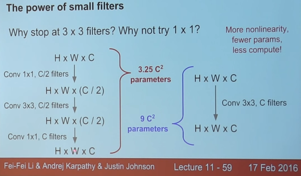
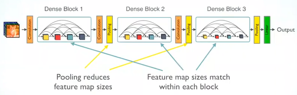
DenseNet
- Densely Connected Convolutional Networks
- img source
- layer output = BatchNorm -> ReLU -> 3x3 conv with k filters => k channels => HxWxk
- concat previous layer outputs to each subsequent layer = +k channels at each layer
- less params than CNN Resnet:
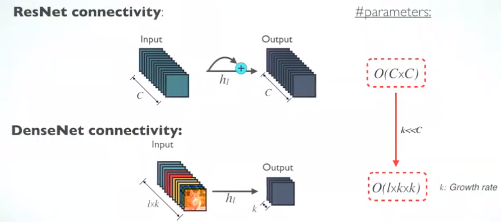
- after each block of L layers:
- reduce number of channels to k = use 1x1 conv with k filters
- reduce filter size by pooling